How to create a dropdown menu in Excel

Firstly, write a list of all the items you would like in your drop down menu. This should be done in a table. If it is not, select the range of cells and press CTRL+T to convert it to a table.

​​​​​​​Now, select the cell on the worksheet where you want your dropdown menu to be. This will usually be the cell that contains the list header e.g. 'Cars'.

Once your list has been created, select data validation under the data tab.

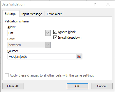
​​​​​​​This will open the data validation menu. Under settings, change the validation style from 'allow' to 'list'.

Next, click in the source box and select the range of cells on your workbook that contain your list of data that is to be used for dropdown menu. Make sure to not select your list header as this will later house the items for your menu.

​​​​​​​The two checkboxes on the right-hand side, in-cell drop down must be checked. Ignore blank is personal preference depending on whether you allow people to leave the cell blank or not.

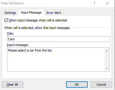
Switch to the Input Message tab, this is where you can define a message to appear when the dropdown menu is clicked. If you wish to add a message, check the ‘show input message when cell is selected ‘ checkbox.
Your message can be entered in the input message box below and be a maximum of 255 characters. A message is optional, if you do not wish to add one, leave the box unchecked.

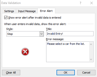
Optionally, to add an error message to your dropdown menu, switch to the error alert tab. Here, check the ‘Show error alert after invalid data is entered’. Choose a style to use to display a warning Icon. Finally, enter a title and error